
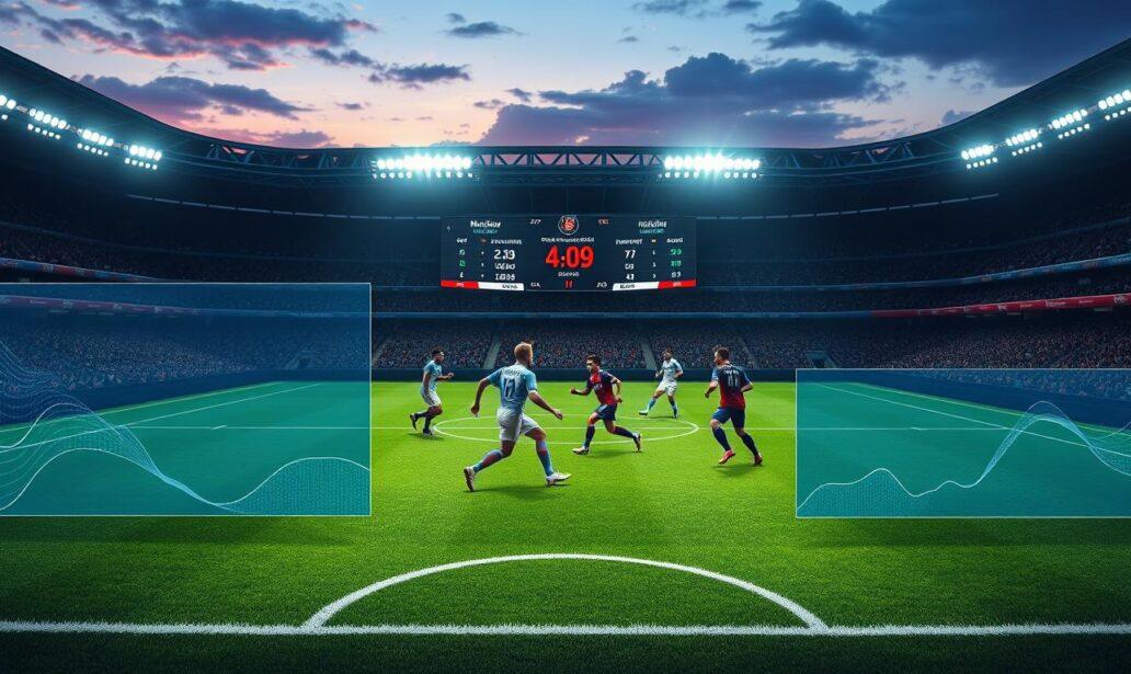
In the fast world of football, knowing the match’s dynamics is key for good analysis. Old models often miss the mark because they don’t get the live action. That’s where the Markov chain comes in. It’s a statistical tool that breaks down a game into clear states, like when a team has the ball or scores a goal.
The Markov Property makes things simpler. It says the chance of moving to a future state only depends on the current state, not past events. This makes it easier to figure out probabilities and adjust to changes during the game.
Using this method, we can keep updating our predictions as new data arrives. This gives us a big edge in live betting. It’s turned in-play betting into a precise, scientific field. For more on related ideas, see our look at the Monte Carlo method.
Define match states and transitions
To use Markov chains well, you need to define match states and their transitions. This step is key to making models that can forecast game results. By knowing how teams move between states, analysts can gain insights into the game’s dynamics.
Core state definitions across sports
Different sports have their own match states, shaped by their rules and gameplay. For example, in football, important states include:
- Possession with Team A
- Possession with Team B
- Goal Scored by Team A
- Goal Scored by Team B
- Match Ended
These states are vital in a Markov chain. They help analysts figure out how likely transitions are, based on past data. In basketball, states might include shot clock status and who has the ball. Hockey might look at even-strength versus power-play situations.
Possession, field zone, and game context states
When setting up match states, think about three main areas: possession, field zone, and game context. Possession shows which team has the ball. Field zones are divided into defensive, midfield, and attacking thirds, or similar in other sports. Game context includes score difference, time left, and player penalties.
Finding the right balance is key. Too few states might not be predictive enough. Too many can make data too scattered, leading to unreliable estimates. Domain knowledge is essential here, making sure the model captures the sport’s tactics without fitting too closely to sparse data.
Also, absorbing states are important. These are final states, like the end of a period or match, that help anchor the model. By looking at transitions between these states, we can forecast things like total goals or comeback chances.
| State | Description | Example Transition |
|---|---|---|
| Possession with Team A | Team A controls the ball | Team A loses possession |
| Goal Scored by Team A | Team A scores a goal | Match resumes with Team B possession |
| Match Ended | Game concludes | N/A |
Estimate transition matrices from play‑by‑play
Estimating transition matrices starts with detailed play-by-play data analysis. This step is key to creating models that predict match outcomes. By understanding possession and scoring probabilities, we can guide our betting strategies.
Getting the data is the first step. Companies like Opta, Sportradar, and Stats Perform provide detailed event feeds. These feeds track every important moment in a match, like passes, shots, turnovers, and goals. This rich data helps us see how teams interact.
Data sourcing and preprocessing
After getting the data, we need to prepare it. This means mapping raw event codes to our state space. We also handle missing or unclear data that might come up during the game. Making sure our analysis is consistent by normalizing for different match lengths and styles is important.
Maximum likelihood estimation and smoothing
The main method for finding our transition matrix is maximum likelihood estimation. Each part of the matrix shows the chance of moving from one state to another. For example, if Team A has the ball, they score 10% of the time. If they lose it, Team B gets it 82% of the time.
To fix the zero-count problem, we use smoothing methods. Methods like Laplace smoothing, Bayesian priors, or hierarchical shrinkage help. They make sure even rare transitions are counted right.
The quality of our transition matrix depends on the data size and our stationarity assumptions. As we continue, we’ll see how these factors affect our predictions.
Time‑dependent/inhomogeneous Markov variants
Live sports are always changing, and models need to keep up. Traditional Markov chains assume the same transition probabilities all game long. But, this doesn’t work well in key game moments.
Why stationary assumptions fail in live sports
Live sports change fast. For example, a team behind by one goal in the last minutes acts differently than when it’s tied. A fixed transition matrix can’t capture this.
Incorporating clock, score, and situational covariates
Inhomogeneous Markov models get around this by changing transition probabilities based on time, score, and other factors. For example, Stats Perform’s model uses fixed time windows, like the next 10 seconds, to improve accuracy and clarity.
There are two main ways to use these models. One is to divide time into chunks and create separate transition matrices for each. The other is to use models where transition odds change with continuous factors. Both make predictions better for live betting.
Even though these models have more parameters, techniques like regularization keep them efficient. This means the transition matrix changes as the game goes on, making simulations more realistic for live betting.
Compute live win probability
We use Markov Chains to find live win probabilities. This method helps us turn the transition matrix into useful estimates. By looking at the current match state, like who has the ball and the score, we can predict the outcome.
Forward simulation and absorbing state analysis
Each simulation run goes through transitions based on the probability matrix. It stops when it hits an absorbing state, meaning the game is over. By combining results from many simulations, we can figure out the win probability for each team and the chance of a draw.

Every event, like a goal or a turnover, starts a new simulation. This keeps the probabilities up to date. It shows how each action affects the game, similar to how possession value models work.
These live probabilities are key for real-time odds. It’s important to think about how to make them accurate and fast. The Markov framework is great for this because it only needs the current state to make predictions.
For more on this, check out the detailed lecture notes.
Kalman filter for drifting strength
In sports analytics, the Kalman filter is a key tool for measuring team strength. It fixes a big problem with old models: they assume team strength never changes. But, injuries, new tactics, and mental factors can change how well a team does.
The Kalman filter uses a Bayesian framework to guess a team’s true strength. It looks at things like how well shots are taken and how much control a team has. This helps analysts keep their views on team ability up to date, which is great for betting.
State‑space representation of team ability
The way team ability is shown involves two main parts: the transition and observation equations. The transition equation shows how a team’s true strength changes over time. It’s like a small step in a random walk.
The observation equation links what we see to the team’s true strength. It includes some noise, or error, in the measurements. This setup lets the Kalman filter get better at guessing team strength as more data comes in.
Observation and transition equations for live updating
As a game goes on, the Kalman filter keeps updating its guess of a team’s strength. It balances what it already knows with new data, taking into account how sure it is of each piece of information. This makes the model more accurate as it goes along.
For instance, if a team’s estimated strength is higher than expected, it might start scoring more. This flexibility is key in live sports, where past data might not always match the current game.
| Factor | Impact on Team Strength | Example |
|---|---|---|
| Injuries | Decrease | Star player out |
| Tactical Changes | Increase/Decrease | Switching formations |
| Fatigue | Decrease | Long matches |
| Psychological Factors | Increase/Decrease | Winning streaks |
Data latency and market microstructure
In live sports betting, how fast data is captured affects your strategy. Knowing about data latency is key for live betting success. This part talks about the challenges of using state-space models where speed is everything.
Data latency comes from several places. First, there’s the time it takes for an event to be caught by optical systems. Then, there’s the delay in processing these events into meaningful actions. Lastly, the time it takes for this data to reach the model server adds more delay. All these delays affect how quickly bettors can act.
For example, big data providers like Opta have feeds that are 2 to 5 seconds late. But systems like Second Spectrum or Hawk-Eye can be under a second. Knowing these differences is important for anyone dealing with real-time pricing.
Feed timing, processing delays, and stale states
Stale states are a big deal here. If a model uses old data, it can be beaten by others who act faster. This shows how important speed is in live betting.
Market microstructure from finance shows how fast getting new info into prices is key. Using tracking data to predict events can give a big advantage in live betting.
Beating the market close with speed and accuracy
You don’t have to be the absolute fastest. Just be quicker than the bookmaker’s changes. By knowing the latency of different data and how bookmakers use it, you can find chances to win. These chances let you spot mispriced lines before they get fixed.
In short, getting good at data latency and market microstructure can give you an edge in live sports betting. Speed, accuracy, and knowing how to use real-time pricing are all key to success in this fast-paced world.
Pricing examples across sports
The impact of state transitions on sports betting pricing is deep and complex. Each sport has its own special dynamics. Understanding these can help make better betting choices.
By looking at specific examples, we see how the transition matrix affects live odds. It’s a key factor in pricing.
Football: next-goal and match outcome markets
In football, a key moment can change the game’s direction. For example, a through ball in the Premier League can raise scoring chances from 3.3% to 33.9%. This shows the importance of looking at the build-up, not just the final shot.
A simple pass in your own half might not mean much. But a through ball into the box could lead to a goal. The transition matrix captures this change. It helps bookmakers adjust odds for next-goal markets, fixing prices that don’t account for quick changes.
Basketball, hockey, and tennis applications
In basketball, states include who has the ball, the shot clock, and the score. A transition matrix based on NBA data can price live spread and moneyline markets well. It catches momentum shifts that box scores might miss.
Hockey uses states like even-strength, power-play, and empty-net. The transition matrix shows how scoring rates change with manpower advantages. This leads to more accurate live betting odds.
Tennis has a natural Markov structure with states like point scores in games, games in sets, and sets in the match. Transition probabilities come from serve and return win rates. They’re updated as the match goes on.
Each sport shows how the state-space framework brings different betting markets together. It respects the unique tactics of each sport while giving a broad view of how state transitions affect pricing. For more on this, see this research paper.
Backtest vs live market close and CLV
Backtesting models against live market data shows their predictive power. This is key for checking state-space models before using real money. The Closing Line Value (CLV) is a key metric here. It shows the difference between the bet odds and the final closing line, which is the market’s best guess.
A model that beats the closing line has a real edge. It finds valuable info before the market does. We test models over many seasons, making live probability estimates at each step. These are then compared to betting exchange prices or bookmaker closing lines.
Methodology for Evaluating Model Performance
We look at mean CLV in basis points and how often bets beat the close. We also check if the edge is real using t-tests or bootstrap procedures. It’s important to avoid biases like survivorship bias and data snooping to make sure our results are solid.
Testing models in different leagues and seasons is key. A model that often has positive CLV can spot bets where the market is wrong. This is like using our Value Detection tool, which compares SportBot’s AI odds to bookmaker prices.
Closing Line Value as the Gold Standard Metric
It’s important to know the difference between statistical and economic significance. A model might have statistically reliable CLV but not make enough money after costs and margins. So, we need to set standards for what makes a good bet in today’s betting markets.
Implementation roadmap
Creating a top-notch in-play modeling system needs a clear plan. First, read match data from a trusted source. Use APIs from Opta or Sportradar for live insights. Look for teams or players with high-PV actions to gain an edge.
Then, compare AI predictions with market odds. If your model shows a higher chance than bookmakers, it’s a sign of value. Use your AI Sports Desk to set alerts for big odds changes on key matches.
In the next step, work on model training. Use past data to set up the state-space. Use smoothing and Kalman filter adjustments for better accuracy. Start with one sport and add more complexity later.
Next, move to live deployment. Package your model with Docker. Make your simulation engine fast, using Rust or C++. Create a layer to turn probabilities into fair prices, keeping a margin you can adjust.
Lastly, link up with betting systems. Connect to exchange APIs or odds services. Use the Kelly criterion for betting. Keep an eye on how well your model does and how fast it is. Start small, test, and grow your system to more sports and bets.