
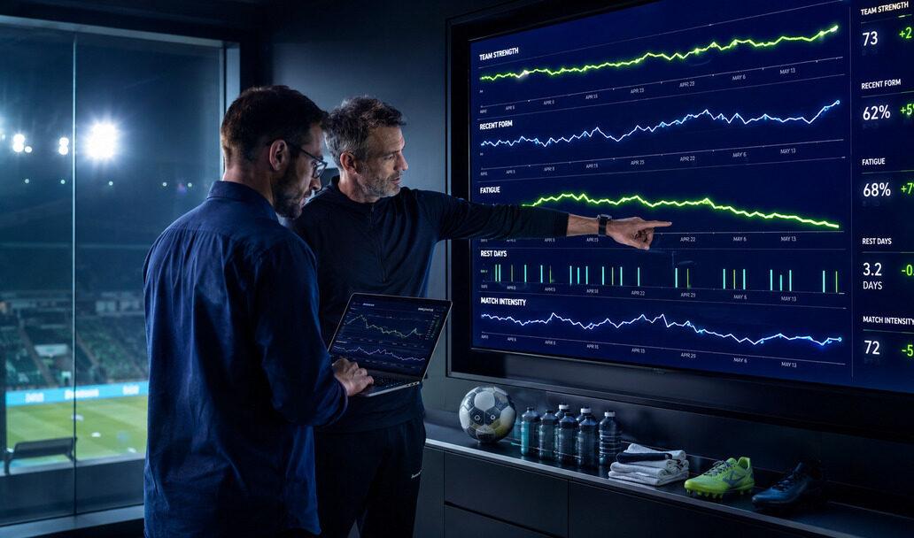
In competitive sports, team performance is more than just one game. Every match, training, and rest period adds to a stream of data. This data is connected, making it key to see team strength as a time-series issue.
Looking at weekly ratings as just numbers misses the point. A team on a winning streak has different momentum than one with the same record but uneven results. Time-series models help catch these important details that other methods miss.
Teams also see ups and downs in performance due to injuries and new strategies. Spotting these changes helps us understand and analyze their data better. This article will show how to use time-series and regime-switching models to spot form and fatigue in team sports.
EWMA vs ARIMA for smoothing
When it comes to smoothing performance metrics, two popular methods stand out: EWMA and ARIMA. Both are key in pulling out useful signals from noisy data.
Exponentially Weighted Moving Averages (EWMA) give more weight to recent data. This means recent games have more impact on current ratings than older ones. The smoothing parameter, λ, controls this rate. Finding the right λ is a matter of careful testing, not guesswork.
ARIMA models, on the other hand, break down time-series data into three parts: autoregressive, integration, and moving average terms. It’s great at catching complex patterns, like those in fixture difficulty or seasonal fatigue.
Choosing between EWMA and ARIMA isn’t simple. You should test both on holdout data and compare their performance. A mix of both can often lead to the best results. Using EWMA for quick updates and ARIMA for deeper insights can give you more accurate team strength estimates.
| Method | Strengths | Considerations |
|---|---|---|
| EWMA | Quick adaptation to recent changes | Requires careful λ selection |
| ARIMA | Models complex dependencies | More complex to implement |
| Hybrid Approach | Combines strengths of both | May require more data |
In conclusion, both EWMA and ARIMA are useful for smoothing team form. For more on ARIMA models, see this detailed whitepaper.
Hidden‑Markov hot/cold regimes
The hidden Markov model (HMM) is a key tool for understanding sports performance. It helps spot hidden performance states that affect game results. A team’s true state—whether they’re on a hot streak, cold spell, or neutral—is not seen directly.
What we see are game results and performance metrics. These come from latent states. The model finds two important matrices:
- Transition Matrix: This shows how teams move between states over time.
- Emission Matrix: This tells us the likely outcomes based on each hidden state.
For example, a team in a hot streak might have expected goal differentials of +0.8 with little variation. But in a cold spell, this could drop to -0.3 with more variation. HMMs are great at spotting when teams are about to change their performance.
When the model shows a team is likely to move from hot to neutral, we can predict a drop in performance. To work well, these models need the right number of states and must be tested with new data.
The hidden Markov model does more than smooth out ratings. It gives a chance of what state a team is in. This helps teams make better tactical and strategic choices, giving them an edge.
| Regime Type | Expected Goal Differential | Variance |
|---|---|---|
| Hot Streak | +0.8 | Low |
| Neutral Phase | 0.0 | Medium |
| Cold Spell | -0.3 | High |

Schedule and rest adjustments
Understanding how rest and match schedules affect fatigue is key for analyzing performance. The role of fixture congestion and rest days on player performance is huge. Teams face big challenges when playing many matches close together.
This can make a big difference in how ready they are compared to opponents who have rested more.
Studies show that muscle fatigue lasts longer than we think. For example, vertical jump performance can stay low for up to 72 hours after exercise. Squat jumps need 72 hours to recover, and other jumps might take even longer. This shows that fatigue accumulation is very important in judging team strength.
To really understand team performance, we need to use schedule-adjusted ratings. These ratings look at how long it’s been after the last game, travel distance, and the load from recent games. When a team plays its third game in seven days, they face different physical challenges than a well-rested opponent.
Here’s a summary of the impact of rest days on performance:
| Days After Last Match | Performance Impact | Recommended Recovery |
|---|---|---|
| 0-24 hours | High fatigue, big drop in performance | 72 hours |
| 24-48 hours | Moderate fatigue, less effective | 72 hours |
| 48-72 hours | Less fatigue, close to normal performance | 96 hours for full recovery |
| 72+ hours | Best performance | Keep up regular training |
In conclusion, momentum can also affect how rest periods work. A team winning streak can give them a mental boost that helps with fatigue. But, the physical limits are real. So, any good model for team strength must include these adjustments. Teams playing on short rest usually don’t meet their expected ratings, showing the importance of considering rest days in performance evaluation.
Forecast horizons and uncertainty bands
The way forecast horizons and uncertainty bands work together is key for sports analysts. In team sports, knowing these concepts helps make better decisions. Point predictions of team strength often don’t cut it, as analysts need forecast distributions with clear uncertainty bands.
The forecast horizon greatly affects model choice and uncertainty band width. For short-term forecasts, like next week’s match, recent performance is key. These forecasts often use Exponentially Weighted Moving Average (EWMA) or short-memory ARIMA components.
As the forecast horizon gets longer, like for the rest of the season or a tournament, other factors matter more. These include squad depth, fixture difficulty, and historical trends. This means models need to handle long-term trends and changes in team performance.
As the forecast horizon grows, so do the uncertainty bands. For example, a single match might have a ±0.5 expected goals prediction interval. But a season-long forecast could have a ±8 points interval in the league table.
Team sports forecasts have asymmetric bands because outcomes are bounded. The impact of tactical decisions when leading or trailing adds complexity. Monte Carlo simulations are best for showing forecast reliability by spreading uncertainty through the model.
Analysts should always report 50%, 80%, and 95% prediction intervals. This helps coaches and decision-makers understand the confidence level of forecasts. Without uncertainty bands, a forecast is just a guess in disguise.
| Forecast Horizon | Prediction Interval | Uncertainty Width |
|---|---|---|
| Single Match | ±0.5 Expected Goals | Narrow |
| Weekly Forecast | ±2 Expected Goals | Moderate |
| Season Projection | ±8 League Points | Wider |

Blend ratings with time‑series signals
Blending ratings with time-series signals is key to understanding team performance fully. It mixes the best of traditional ratings with the quick insights of time-series analysis. This mix makes forecasts more accurate than either method could on its own.
Ensemble methods are vital in this blend. They combine different machine learning models like gradient boosting and neural networks. Each model predicts stamina and fatigue using deep learning features. This ensemble architecture improves predictions by covering all angles of complex data.
Using a hybrid forecasting model is smart. For example, Elo-based ratings give a solid foundation of team quality over time. At the same time, time-series models catch up on recent trends and changes. The way these are blended can vary:
- A weighted average where the time-series part gets more weight when things get volatile.
- A Bayesian setup where the rating acts as a starting point, updated by new data.
- A machine learning model that finds the best mix from past data.
Research backs this method. Studies show mixing predictions leads to better fatigue forecasts than one model alone. The same goes for team strength predictions. Ratings show a team’s core strength, while time-series signals track recent changes.
A model that uses both does better than any single method. This is true, even more so when teams are changing their game. The weights for blending should change too. The time-series part should get more weight when recent results differ a lot from what the rating suggests.
Walk‑forward validation and CLV lift
Walk-forward validation is key for checking how well time-series models work. It’s a strict out-of-sample testing method. It makes sure predictions are made with data available at the time.
This method is different from random data splitting. Walk-forward validation uses all data up to a point to train the model. Then, it predicts the next period and moves the training window forward. This way, it better reflects real-world performance.
Just looking at how accurate a model is isn’t enough. We need to see if it adds value. Customer Lifetime Value (CLV) lift shows the extra benefits of using the model. In sports betting, it’s about making more money than expected. For team management, it helps make better player rotation decisions.
It’s also important to find and fix any biases in the model. If a model always overestimates or underestimates team strength, we need to fix it. For example, bias can be found by looking at the average error in the data:
- B_stamina = (1/N) Σ (Ŝ(t) – S_true(t))
Looking at how the model performs at different times in the season is also key. A model that does well in walk-forward validation and has positive CLV lift is ready for use.
For more on statistical modeling, see the basics of statistical modeling.
Deployment cadence during season
Having a good deployment cadence during the season is key for team success. How often and when to update model updates is a big decision. It can make a team’s analysis better or worse.
For sports with games every week, updating team strength after each game is best. This rhythm helps teams make quick in-season adjustments. A strong deployment pipeline is needed to handle new data smoothly.
Real-time monitoring from athlete tracking shows the importance of quick feedback. If a player gets hurt or a team does poorly in certain areas, the model should notice right away. This quick adjustment is key to staying ahead.
Version control and model registry help make sure every strength estimate is reliable and can be checked. The deployment schedule should also consider big changes in the season, like transfer windows or coaching changes. These times are great for updating the model.
A consistent deployment plan, with room for updates when needed, is essential for reliable team strength analytics. Following these steps helps teams stay quick and responsive all season.
Monitor drift and set alerts
Drift monitoring is vital for keeping predictive models working well. In a changing environment, data can shift due to many reasons. This includes changes in rules or team dynamics. It’s important to check how well models perform regularly to avoid mistakes in team strength estimates.
To keep an eye on drift, try these strategies:
- Track Prediction Errors: Watch how prediction errors change over time. Compare them to a baseline from a validation period.
- Set Alert Thresholds: Create alert levels. For example, if the mean absolute error goes up by a certain percentage, alert someone.
- Utilize a 3% Deviation Flag: Use the 3% deviation from neuromuscular fatigue monitoring as a guide for errors.
- Monitor Regime Transition Probabilities: Keep an eye on how likely the model is to switch between regimes. This can show if the model is off.
- Address Bias Accumulation: Look for consistent drift in one direction. This means the model is not catching changes in the game.
It’s important to find the right balance for alert levels. If they’re too strict, you might get too many false alarms. If they’re too loose, real problems might be missed. To improve monitoring, link automated retraining to drift alerts. But, always have a human check to tell real issues from temporary problems.
Roadmap and resources
Creating effective time-series models for team strength analysis needs a clear plan. Start by setting up a strong data system. You need reliable ways to get match results, player info, and schedules. Python libraries are key here. Use statsmodels for ARIMA and exponential smoothing, and hmmlearn for hidden Markov models.
The process has five steps. First, use EWMA and ARIMA for baseline models. Then, test them with walk-forward techniques. Next, add hidden Markov models for regime-switching, adjusting states as needed.
After that, include schedule and rest adjustments for fixture congestion. Then, create an ensemble that mixes ratings with time-series signals. This blends different data types.
Lastly, set up the system for automated monitoring and alerts. Each step should be tested before combining everything. Tools like sportype and soccerdata offer valuable match data. Investing in these resources improves your models over time. As new data and methods come along, your team will stay ahead in analysis.